Production theory basics
|
|
In microeconomics, Production is simply the conversion of inputs into outputs. It is an economic process that uses resources to create a commodity that is suitable for exchange. This can include manufacturing, storing, shipping, and packaging. Some economists define production broadly as all economic activity other than consumption. They see every commercial activity other than the final purchase as some form of production.
Production is a process, and as such it occurs through time and space. Because it is a flow concept, production is measured as a “rate of output per period of time”. There are three aspects to production processes:
- the quantity of the commodity produced,
- the form of the good produced,
- the temporal and spatial distribution of the commodity produced.
A production process can be defined as any activity that increases the similarity between the pattern of demand for goods, and the quantity, form, and distribution of these goods available to the market place.
| Contents |
Efficiency and X-efficiency
A production process is efficient if a given quantity of outputs cannot be produced with any less inputs. It is said to be inefficient when there exists another feasible process that, for any given output, uses less inputs. Some economists (in particular Leibenstein) use the term X-efficiency to indicate that production processes tend to be inherently inefficient due to satisficing behaviour. The “rate of efficiency” is simply the amount of (or value of) outputs divided by the amount of (or value of) inputs. If a production process uses 50 units of input (or $5000 worth of inputs) to produce one unit of output it is more efficient than a process that uses 55 units of input (or $5500 worth of inputs) to produce the same level of output. It is said to be 10% more efficient ({55-50}/50=1/10=10%).
Factors of production
The inputs or resources used in the production process are called factors by economists. The myriad of possible inputs are usually grouped into four or five categories. These factors are:
- Raw materials (natural capital)
- Labour services (human capital)
- Capital goods
- Land
Sometimes a fifth category is added, entrepreneurial and management skills, a subcategory of labour services. Capital goods are those goods that have previously undergone a production process. They are previously produced means of production. Some textbooks use "technology" as a factor of production.
In the “long run” all of these factors of production can be adjusted by management. The “short run” however, is defined as a period in which at least one of the factors of production is fixed. A fixed factor of production is one whose quantity cannot readily be changed. Examples include major pieces of equipment, suitable factory space, and key managerial personnel. A variable factor of production is one whose usage rate can be changed easily. Examples include electrical power consumption, transportation services, and most raw material inputs. In the short run, a firm’s “scale of operations” determines the maximum number of outputs that can be produced. In the long run, there are no scale limitations.
Total, average, and marginal product
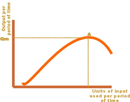
The total product (or total physical product) of a variable factor of production identifies what outputs are possible using various levels of the variable input. This can be displayed in either a chart that lists the output level corresponding to various levels of input, or a graph that summarizes the data into a “total product curve”. The diagram shows a typical total product curve. In this example, output increases as more inputs are employed up until point A. The maximum output possible with this production process is Qm. (If there are other inputs used in the process, they are assumed to be fixed.)
The average physical product is the total product divided by the number of units of variable input employed. It is the output of each unit of input. If there are 10 employees working on a production process that manufactures 50 units per day, then the average product of variable labour input is 5 units per day.
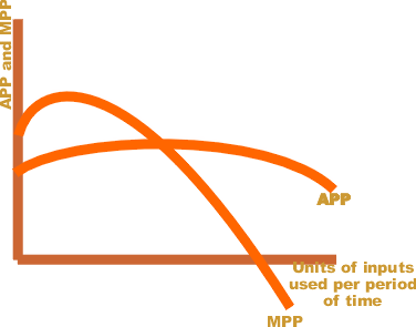
The average product typically varies as more of the input is employed, so this relationship can also be expresses as a chart or as a graph. A typical average physical product curve is shown (APP). It can be obtained by drawing a vector from the origin to various points on the total product curve and plotting the slopes of these vectors.
The marginal physical product of a variable input is the change in total output due to a one unit change in the variable input (called the discrete marginal product) or alternatively the rate of change in total output due to an infinitesimally small change in the variable input (called the continuous marginal product). The discrete marginal product of capital is the additional output resulting from the use of an additional unit of capital (assuming all other factors are fixed). The continuous marginal product of a variable input can be calculated as the derivative of quantity produced with respect to variable input employed. The marginal physical product curve is shown (MPP). It can be obtained from the slope of the total product curve.
Because the marginal product drives changes in the average product, we know that when the average physical product is falling, the marginal physical product must be less than the average. Likewise, when the average physical product is rising, it must be due to a marginal physical product greater than the average. For this reason, the marginal physical product curve must intersect the maximum point on the average physical product curve.
Diminishing marginal returns
These curves illustrate the principle of diminishing marginal returns to a variable input (not to be confused with diseconomies of scale which is a long term phenomenon in which all factors are allowed to change). This states that as you add more and more of a variable input, you will reach a point beyond which the resulting increase in output starts to diminish. This point is illustrated as the maximum point on the marginal physical product curve. It assumes that other factor inputs (if they are used in the process) are held constant. An example is the employment of labour in the use of trucks to transport goods. Assuming the number of available trucks (capital) is fixed, then the amount of the variable input labour could be varied and the resultant efficiency determined. At least one labourer (the driver) is necessary. Additional workers per vehicle could be productive in loading, unloading, navigation, or around the clock continuous driving. But at some point the returns to investment in labour will start to diminish and efficiency will decrease. The most efficient distribution of labour per piece of equipment will likely be one driver plus an additional worker for other tasks (2 workers per truck would be more efficient than 5 per truck).
Resource allocations and distributive efficiencies in the mix of capital and labour investment will vary per industry and according to available technology. Trains are able to transport much more in the way of goods with fewer "drivers" but at the cost of greater investment in infrastructure. With the advent of mass production of motorized vehicles, the economic niche occupied by trains (compared with transport trucks) has become more specialized and limited to long haul delivery.
Many ways of expressing the production relationship
The total, average, and marginal physical product curves mentioned above are just one way of showing production relationships. They express the quantity of output relative to the amount of variable input employed while holding fixed inputs constant. Because they depict a short run relationship, they are sometimes called short run production functions. If all inputs are allowed to be varied, then the diagram would express outputs relative to total inputs, and the function would be a long run production function. If the mix of inputs is held constant, then output would be expressed relative to inputs of a fixed composition, and the function would indicate long run economies of scale.
Rather than comparing inputs to outputs, it is also possible to assess the mix of inputs employed in production. An isoquant (see below) relates the quantities of one input to the quantities of another input. It indicates all possible combinations of inputs that are capable of producing a given level of output.
Rather than looking at the inputs used in production, it is possible to look at the mix of outputs that are possible for any given production process. This is done with a production possibilities frontier. It indicates what combinations of outputs are possible given the available factor endowment and the prevailing production technology.
Isoquants
There are many ways of producing a given level of output. You can use a lot of labour with a minimal amount of capital, or you could invest heavily in capital equipment that requires a minimal amount of labour to operate, or any combination in between. For most goods, there are more than just two inputs. For example in agriculture, the amount of land, water, and fertilizer can all be varied to produce different amounts of a crop. An isoquant, in the two input case, is a curve that shows all the ways of combining two inputs so as to produce a given level of output. In the three input case it will be a surface. Iso is Latin for equal and quant is short for quantity. Movement along an isoquant depicts a constant rate of output, but a changing input ratio. A unique isoquant can be constructed for every level of output, and a family of isoquants can be created to represent various output levels. Isoquants further from the origin represent greater amounts of output. Isoquants are usually considered to be everywhere dense, meaning an infinite number of them could be plotted in any two input space.
Isoquant_small.png
alt text
Isoquant
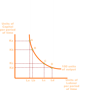
A typical isoquant is illustrated in the diagram to the right. At point A in the diagram Ka unit of capital is combined with La units of labour to produce 100 units of output. It is downward sloping, convex to the origin, and non-intersecting (additional isoquants, not shown, would be drawn parallel to this one). A complete isoquant is actually a closed curve, but only the “down sloping to the right” portion makes economic sense. The upward sloping parts of isoquants, for example, indicate that that level of output could be produced by less of both inputs so this section is of little interest to decision makers. The economic section of the isoquants is defined by a pair of lines called ridge lines.
The “downward to the right” slope of the economic region of an isoquant is due to the possibility of substituting one input for another in the production process while keeping the level of output constant.
The marginal rate of technical substitution
Isoquants are typically convex to the origin reflecting the fact that the two factors are substitutable for each other at varying rates. This rate of substitutability is called the “marginal rate of technical substitution” (MRTS) or occasionally the “marginal rate of substitution in production”. It measures the reduction in one input per unit increase in the other input that is just sufficient to maintain a constant level of production. For example, the marginal rate of substitution of labour for capital gives the amount of capital that can be replaced by one unit of labour while keeping output unchanged.
To move from point A to point B in the diagram, the amount of capital is reduced from Ka to Kb while the amount of labour is increased only from La to Lb. To move from point C to point D, the amount of capital is reduced from Kc to Kd while the amount of labour is increased from La to Lb. The marginal rate of technical substitution of labour for capital is equivalent to the absolute slope of the isoquant at that point (change in capital divided by change in labour). It is equal to 0 where the isoquant becomes horizontal, and equal to infinity where it becomes vertical.
The opposite is true when going in the other direction (from D to C to B to A). In this case we are looking at the marginal rate of technical substitution capital for labour (which is the reciprocal of the marginal rate of technical substitution labour for capital).
It can also be shown that the marginal rate of substitution labour for capital, is equal to the marginal physical product of labour divided by the marginal physical product of capital.
In the unusual case of two inputs that are perfect substitutes for each other in production, the isoquant would be linear (linear, a straight line, with a function y = a - bx). If, on the other hand, there is only one production process available, factor proportions would be fixed, and these zero-substitutability isoquants would be shown as horizontal or vertical lines.


